Calculation of Object Size
Knowing distance as a function of size and having determined number of screen pixels per degree from the montage of images, one can then calculate the dimensions of the object. E.g., when the object was calculated to be 5.74 miles distant, its width was 20 pixels. There were about 350 pixels/deg. Therefore the object was 20/350 = .057 deg. At the given distance, each degree was 0.1 mile or 530 feet. Therefore the object calculates to .057 x 530 = 30 feet wide.
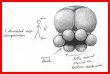
Averaging over several dozen such values, the mean width turned out to be 28.4 feet. The same calculation for the height gave 25.0 feet average. Error is probably ± 10%. (Scaled image at right)
These values are about double what I previously calculated when I was going by the (erroneous) radar range data of the smallest images at the beginning of the video and doing measurements with a ruler off a TV screen, rather than from a digitized video and screen captures. At that time I got about 15-16 wide and 9-10 feet thick. These values should now be considered outdated.
By comparison, Martin Powell, also using measurements off a TV screen and slightly larger images when the radar range values were deemed reliable, came up with a height of 8.7m ± 2.5. or 28.5 ft ± 8.2, and width/lengths of 11.6m ± 3.5 and 12.3m ± 3.7 or 38.0 ft ± 12.1 and 40.3 ft ± 12.8. The dimensions are in basic agreement at the lower ends of his error estimates.
For further comparison, a similar multi-lobed Gulf Breeze object was estimated by Dr. Bruce Maccabee as 30 x 20 feet, by comparing it to a nearby F-15 jet interceptor in the same picture (to scale properly, an F-15 is about 64 feet long).
Similarly, for the object videoed by Stan Romanek over Denver in 2000, Romanek included a drawing of the object with a stick-figure person next to it for scale. This object, according to this drawing, would have been approximately 12 feet high and 15 feet wide.
Another multi-lobed object, just photographed Sept. 11, 2002, also appears to be relatively small in size, though not possible to scale accurately (images are copyrighted and can't be reproduced here). At one point, however, it is partly obscured by a near-by streetlight, possibly about 100 feet away and 1 foot in width. The object has an angular width about 2/3rd's that of the light. If we assume from the clarity of the object and lack of haze that it was roughly 1/2 mile from the camera, then its diameter would be in the vicinity of 18 feet, very roughly. If were 3/4 mile distant, then it would be about 27 feet across.
Based on this small sample, these various multilobed UFOs seem to be relatively small, under 30 feet in width.
Graphical Results
OVERALL 3D TRAJECTORY: This shows a 3-D plot of the UFO trajectory from the point of view of the S-30 radar/camera site (yellow sphere foreground). The UFO is modeled as four spheres in a tetrahedral structure, and is enlarged 15 times for clarity. Each grid square represents 1/2 mile on a side. South is left, North right (red grid lines), and West into the screen (green grid lines). The video begins with the UFO far in the distance (~9.8 miles) at left, moving sideways, and about 1000 feet above ground level. Black Mt. is in the background about 23 miles distant. After executing a sharp turn about 20 seconds into the video, the object rapidly accelerates and starts climbing, quickly approaching the camera. It crosses due West of S-30 2 minutes later, for an average speed of about 300 miles per hour. At this point it is only about 2 miles from S-30. At the end of the video at far right, UFO is about 7500 feet above S-30, headed North, and traveling about 240 mph. The gap in the trajectory near the Sun is caused by the UFO getting lost in the Sun's glare. The trajectory is projected onto the black vertical grid lines in the background (red dots) to show the UFO's vertical trajectory, further detailed in other graphics below. Note several distinct regions of climb followed by leveling out. The trajectory is also projected onto the ground (blue dots) to show the ground trajectory. The white boxed area at far left around Black Mt. is blown up in next graphic.
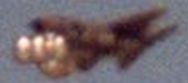
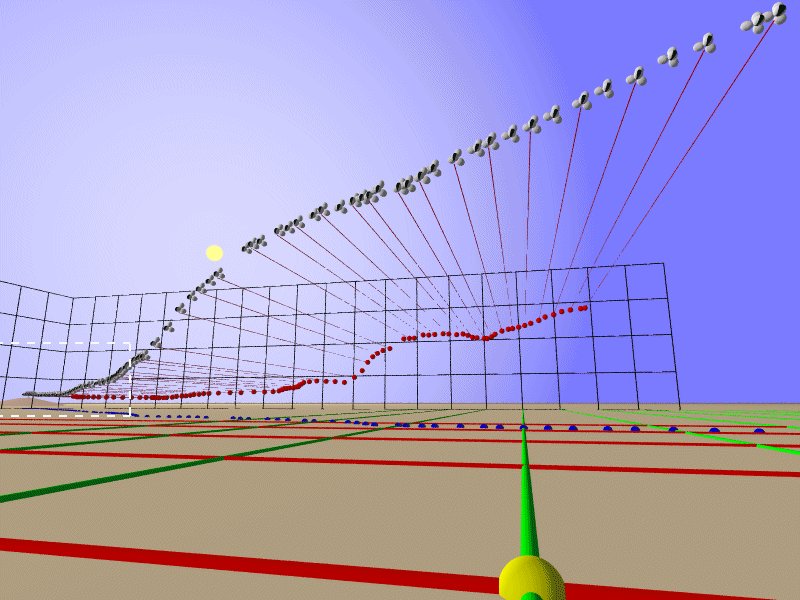
ENLARGED 3D TRAJECTORY: This graphic depicts the 3D trajectory at the beginning of the video when Black Mt. was in the background and the UFO was rising through background cloud layers. This has been superimposed on a montage of dozens of screen captures. (Note: only 50% of original size) The original video UFO appears as a darkish dot most of the time, whereas the recreated UFO shows whitish lobes. Unlike the above graphic, the recreated UFO is shown in "true size" of about 28 feet in width. Note how closely the recreated trajectory follows the original, with the modeled UFO usually falling on top of the original. It is never off by more than 1 or 2 object widths. Degree markers derived from the montage for azimuth and elevation have been added. Also added are some representative values of time, distance, and extremes of velocity. Note at beginning when moving sideways, the object is moving slowly. At about 20 seconds, when it is directly over the peak of Black Mt., it turns and rapidly approaches the camera. Note the rapid acceleration to over 600 mph within a few seconds, followed by several rapid decelerations and accelerations. The object also begins climbing about 40 seconds into the video and is at its maximum rate of climb and acceleration toward the end (right after it suddenly “sprouts” the glowing white lobes).
ANIMATED 3D TRAJECTORY: This animation follows the UFO from the beginning of its trajectory towards the end from the viewpoint of the UFO. Overlaid on top is a shortened transcript of range operator comments plus data on the UFO's calculated speed, altitude, and distance from the camera. Animation speed is four times actual speed. Rotations of the UFO and changes in the appearance ("sprouting" glowing white lobes and shifting blackened lobe) area are also simulated. Requires an Apple Quicktime movie plug-in. (File 2 Megabytes in size)
This details the UFO ground trajectory. Initially heading slowly sideways to the S-30 site at a distance of 9.8 miles, it turns and rapidly heads almost straight for S-30 to the Northeast. At about 79 seconds, when it has approached to within about 2 miles, it suddenly starts veering off to the North. It shows another "kink" in the trajectory, or sudden direction change, at about 130 seconds as it veers off to an almost due North course. Average velocities for intervals between yellow data points are shown alongside the trajectory in blue. Note the multiple large accelerations and decelerations of the object. Various features derived from USGS topo and other maps are also shown, such as other camera sites, communication antennae, practice targets, and monitoring sites. Elevations of two sites that might be called out in the S-30 and S-13 videos are shown, along with "Jerry" site, mentioned in the S-30 video.
GROUND TRAJECTORY/VELOCITY BUBBLE GRAPH: This is a view of the ground trajectory with velocity represented by the width of the “bubble” for each data point. This more vividly shows the wide variations in velocity. The area of the bubble is approximately proportional to the power output. On three occasions, the object rapidly accelerates to high velocity (reaching about 700 mph at one point), then rapidly decelerates to a much lower velocity. This is very anomalous flight performance.
ALTITUDE vs. DISTANCE & SPEED: This more clearly shows how the object rose in altitude with the distance south or north of the camera (red curve). The net speed vs. distance is also shown at the bottom of the plot (purple). There is no overall correspondence between speed and changes of altitude, though in two instances (region between about 1 and 4 miles south) speed increases before the object goes into a climb in altitude. During the climb the speed rapidly drops. It’s as if the object picks up speed and then uses it to “coast” to a higher elevation. However, this isn’t the case for a final climb towards the end where the net speed remains fairly constant. Also near the beginning, the object accelerates to high speed then rapidly slows down but maintains near-level flight.
ALTITUDE vs. DISTANCE & SPEED (bubble plot): This is the same plot but with speed now plotted by "bubble" size, which more graphically illustrates the large variations in speed. Bubble width is proportional to the speed and bubble area approximately proportional to the power or energy output. Again note sudden burst of speed at around 3 miles distance south just before a steep climb and just after lobes on object suddenly start glowing., followed by very rapid drop in speed during climb.
ALTITUDE vs. TIME: This is another view of the altitude changes but plotted against time into the video. Here the steepness of the altitude changes represents rate of climb, while the steepness of the velocity curve represents the rate of acceleration or deceleration. The highest acceleration occurs just before the start of a steep climb around 70 seconds, also corresponding to the steepest absolute angles of climb of about 55 degrees (appearing as 60-70 deg. climb angles from viewpoint of camera), corresponding to one range operator commenting "it's going straight up." This is also when the object suddenly “sprouts’ glowing white lobes on the bottom. Perhaps this is an extra propulsion system being turned on. Details of velocity and acceleration are in the next graph.
VELOCITY vs. TIME: The net velocity of the craft--in yellow-- is plotted along with the component radial velocity --in black-- plus net vertical and horizontal velocities (velocities perpendicular to radial component) —in blue. Note that throughout most of video, the major component of velocity is radial, i.e., towards the camera. Only when the object draws near the camera and passes it to the west does the radial component drop and the perpendicular components (mostly horizontal) start to dominate. This plot again illustrates the sudden darting jumps in velocity peculiar to this craft, with maximum accelerations and decelerations during these jumps noted. There are three such velocity peaks, with maximum velocities near 700 mph, ruling out most conventional aircraft. The maximum acceleration near 10 g is high but not necessarily unconventional. However, the three rapid decelerations after the three main accelerations are anomalous and not typical for a conventional aircraft. The first deceleration, around 6 g (at about 30 seconds), is especially high and not explainable by the craft going into a climb, as associated with the other two decelerations. Instead the craft is in near-level flight at the time (see previous graph). Also plotted is the increase in object size—in red—adjusted for camera zoom (shown as pixels x 10). Overall the object smoothly increases in size as it approaches the camera, except for some “bumps” corresponding to the velocity jumps. This is to be expected, since calculation of velocity was derived from changes in image size.
For about the first 20 seconds of video, the object is just a small blob on the screen with little or no change in size and moving to the right, with Black Mt. in the background. Then it starts to increase in size, indicating that it should be approaching the camera. But between 18 and 27 seconds, the range indicator jumps from 6955 meters to 7485 meters. By 35 sec., the size has clearly increased by about 25%, but the range indicator shows a jump to about 12790 meters (~8 miles). Going strictly by the range indicator, the object would seem to be initially moving away from the camera, but the size increase indicates it's moving towards the camera.
At 49 seconds, the radar return flatlines and the range indicator jumps to over 32000 meter. Between 59 and 61 seconds, the range indicator suddenly drops to 19000 meter, then 9135 meter, where it "freezes" for the remainder of the video. Despite the range indicator indicating over a factor of three change in distance in the space of only 2 seconds, the object again shows little or no change in size.
Overall, the size of the object increases by about 8 times from the start of the video to maximum size, or about 5 times when camera zoom is accounted for. Yet the range has supposedly increased from 6955 meters at the beginning to 9135 meters when the object is 5 times larger in size. Something is obviously very wrong with the range indicator.
Scaling the Distance
To deal with the problem of the erratic radar ranging, I used the relative size of the object as an indicator of the distance. Thus if the object was 5 times bigger towards the end of the video than at the beginning, it was also 5 times closer to the camera.
While this provides the relative distance, it does not give the absolute distance. However, there was one section of radar returns that seemed reliable, when the display showed a strong radar blip between 32 and 49 seconds, and the indicated range consistently decreased at the same time that the object was consistently growing larger in size. I used the indicated range at the beginning of this period as the baseline distance, when the range indicator showed 12795 meters (7.95 miles). All other distances could then be scaled against this distance by comparing relative object size.
One potential problem with this method is the reliability of the object size measurements, particularly when the object is small. E.g., in 640 x 480 digitized video, at the video start the object is typically only about 11 pixels wide. Defining the fuzzy object boundaries is a judgment call, and it is very easy to have differences in width measurements of +/- 2 pixels, or about +/- 20%. But since distance is now being determined by size, this could easily cause seeming jumps in distance of +/- 20%, which would likely be artifactual.
Another potential problem is that the object may not be presenting a constant profile. This is very obvious when the object gets closer. The object is not totally symmetrical and can also be seen to rotate one way and then another. This too can affect measurement of the width.
Another thing that had to be taken into account was camera zoom. There were two such zooms during the video, one at 64 seconds of about 15%, and another at 79 seconds of about another 30%. To keep everything normalized, sizes post-zoom were scaled to pre-zoom sizes using the calculated zoom ratios.
To try to minimize various potential errors, I did a running average of width by averaging the two previous and following measurements with the current one. When doing such averaging there is always the danger that true rapid changes in size, distance, velocity, and acceleration might be missed. But I felt there was too much potential sources of error in determining the range, and it was better to take the more conservative approach. This also has the advantage that if any large variations remain, they are much more likely to be real than artifacts. As it turns out, even with the heavy averaging, there are large swings in velocity and acceleration that are almost certainly real and help define the anomalous nature of the craft.
This approach differs significantly from that used by Martin Powell, who did not determine range point by point, but assumed a straight line trajectory and constant velocity as the object loomed in size. However, with a better handle on the range, it turns out that the velocity is not constant and the trajectory is not straight, although Powell's assumption was a good, first-order approximation.
A confirmation of the overall accuracy of the size/distance method came 113 seconds into the video when one of the range controllers called out the altitude as 11,000 feet (see transcripts). At this time, my calculation showed the object as 2.8 miles distant and 5800 feet above radar/camera. When added to the altitude of the radar/camera (5130 - 5250 feet, depending on the exact position of S-30), the calculated total altitude was 10,930 – 11,050 feet, or essentially an exact hit.
Determining Azimuth and Elevation Angles
Besides range, it is necessary to know the azimuth and elevation angles to get a complete 3-D trajectory and determine other values of interest, such as velocity and acceleration. Seemingly this should be completely straightforward, since these angles are also overlaid on the video and have nothing to do with the radar. They are simply how much the camera/radar mount rotates left/right and up/down.
One problem is that these overlaid screen values are shown only as whole numbers, which lacks the necessary precision. E.g., at the beginning of the video, the elevation angle shows 1 degree for the first 45 seconds before finally increasing to 2 degrees. Yet the elevation angle is obviously increasing for part of this time. Likewise, the azimuth starts off reading 218 degrees, but where is the actual start point for 218 degrees?
Another problem, somewhat unexpected, is that sometimes these values are a little erratic as well, as I discuss a little further below. In the worst example, the indicator flipped from 220 to 221 degrees azimuth, then went back to 220 degrees before eventually settling in at 221. All this period, cloud patterns show that that this wasn't due to reversal of the object, which moved progressively rightward. Instead it was a flaky screen indicator.
I dealt with the imprecision in azimuth and elevation in two basic ways. For about the first 70 seconds of video, I constructed a large montage of dozens of individual frames, using Black Mt. and distant cloud layers as fixed reference points. Among other things, the montage showed that the object trajectory varied smoothly, and that the seemingly sudden direction changes were almost entirely the result of camera jitter while attempting to track the object.
Once the object rose above the reference cloud layers, I assumed for the rest of the video that the trajectory continued to vary smoothly. The object was now much closer and also moving much more rapidly than it was initially. Displayed azimuth and elevation angles were now changing every few seconds instead of tens of seconds. I either tried to select data points where the display flipped angles or, assuming smooth variation, interpolated between angle flips. In practice, usually one or the other angle had to be interpolated because azimuth and elevation angles rarely changed together in the same frame.
Another thing I discovered with the montage is the distance between angle changes was not constant. However, because I was able to determine absolute position with the montage, I was able to average distance between angle change over about 8 degrees in the horizontal direction and 5 degrees in the vertical. This turned out to be about 350 pixels per degree for azimuth and about 330 pixels per degree for elevation in my 640 x 480 digitized video. I then used these averages to try to best-fit azimuth and elevation transition points. Usually these were within 0.1 or 0.2 degree of the screen transitions, as the table below indicates. (Note: numbers in boldface represent screen transition points.)
The table below gives the results for the calculated azimuths and elevations vs. the what was displayed on the screen:
Time Screen Calc. Screen Calc. Comments
(sec.) azim. azim. elev. elev.
(deg.) (deg.) (deg.) (deg.)
_________________________________________________________________
00.0 218 218.1 1 1.1 Video start (23:20:24)
10.8 219 218.9 1 1.2
24.8 220 219.9 1 1.2
35.6 220 221.0 1 1.3 Varied between 220 and 221
40.4 221 221.5 1 1.3 Remained at 221
45.7 221 221.9 2 2.0
46.7 222 222.0 2 2.1
54.7 223 223.2 2 2.7
57.2 224 224.1 3 3.1
64.2 224 224.7 4 4.0
64.8 225 224.8 4 4.1
68.0 225 225.4 5 4.9
68.9 226 225.7 5 5.2
71.2 226 226.1 6 5.9
_________________________________________________________________
To get a feel for the amount of linear error, at the beginning of the video, the distance was 9.83 miles-- every 0.1 degree corresponds to about 90 feet. The width of the object turns out to be about 30 feet (see immediately below). Therefore, even at maximum distance, 0.1 degree error represents only about three object widths.